ARCH

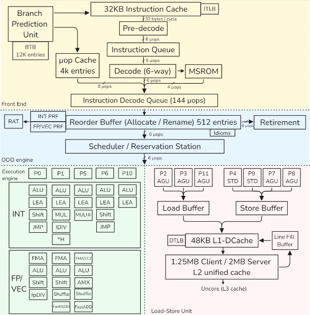
this is a representation of the Golden Cove intel architecture

Dynamic Frequency Scaling (DFS)

Also called Turbo mode.
Allows the CPU to temporarily increase its frequency above the base clock to boost performance.
This can distort benchmarks, since the CPU does not run at a constant frequency, reducing result consistency and accuracy.

Architecture models (high level)

1) Register-based, load–store architectures

Arithmetic ops use registers only
Memory accessed only via explicit load/store
Easy pipelining, OoO-friendly, compiler-friendly
Most modern ISAs

Examples: ARM, RISC-V

2) Register-based, register–memory architectures

Arithmetic ops may use register + memory operand
ISA is not load–store, but microarchitecture behaves like one
Legacy-friendly, complex decoding

Example: x86

Small remark: Stack-based architectures

Operands implicit on a stack
Compact encoding, poor for pipelining
Common in VMs, not modern CPUs

Examples: JVM, WebAssembly

Pipeline

detail cpu pipeline here

PIPELINE Example

add rax, [rbx+8]

1. Frontend — What instruction to run?

BPU predicts next PC
L1 I-cache fetches instruction bytes
Pre-decode finds instruction boundary
Decode → 2 µops:
- µop 1: load [rbx+8]
- µop 2: add → rax
µop cache may bypass decode entirely
µops enter IDQ

2. Rename / Allocate — Prepare execution

ROB allocates entries
RAT maps:
- rax → physical register P42
Dependencies tracked
µops enter Scheduler (RS)

3. Execute — Do work when ready

Load µop

AGU computes rbx + 8 (virtual address)
DTLB translates VA → PA
L1 D-cache lookup
If hit → value ready

Add µop

Waits for load result
Dispatched to INT ALU port
Computes addition

4. Memory system — Handle misses if needed

If L1 miss:
- L2 → L3 → RAM
Fill Buffer tracks request
Load resumes when data arrives

5. Retire — Make it architecturally visible

µops complete out of order
ROB retires in order
rax updated
Instruction committed

6. What each block did (one line each)

BPU: guessed next instruction
Frontend: turned bytes → µops
ROB / RAT: renamed + tracked speculation
Scheduler: waited for operands
AGU: computed address
TLB: translated address
Cache: supplied data
ALU: computed result
ROB retire: committed state

Pipeline Hazards (Reminder)

Break ideal pipelining → stalls
Affect throughput / effective frequency
Fully handled by hardware

Structural

Resource conflict (same unit, same cycle)
Mitigation: more hardware (ALUs, ports)

Data

RAW: true dependency → forwarding
WAR: false dependency → register renaming
WAW: false dependency → register renaming

Control

Branches / flow changes
Mitigation: branch prediction, speculation

A superscalar engine

executes multiple independent instructions per cycle by issuing them to several execution units in parallel.

Branch Prediction

Correct prediction → high throughput
Misprediction → expensive pipeline flush
Uses dynamic, adaptive predictors

Branch Types

Unconditional / direct
- Always taken
- Single target
- Easy to predict
Conditional
- Taken / not taken
- Forward (if/else): often not taken
- Backward (loops): often taken
Indirect
- Multiple targets
- From switch, function pointers, virtual calls
- Returns are also indirect

CACHE

Cache is address-based

Cache does not store variables
Stores data indexed by physical addresses
Any access is:
- Address → set → tag match → hit/miss
cache line (usually 64B, Apple M chips: 128B)

Address generation

Address Generation Unit (AGU):
- base register + offset
Result = virtual address

Addresses used by programs

Load / store instructions issue virtual addresses (VA)
All address generation happens in load–store units
Other execution units do not see addresses

Cache access

Cache stores physical memory only
Cache lines are physically tagged
Allows cache indexing and address translation to proceed in parallel (L1)
L2 / L3 caches require translation before lookup

TLB (Translation Lookaside Buffer)

Purpose

Cache recent virtual → physical translations
Avoid expensive page-table walks

TLB hierarchy

L1 iTLB: instruction fetch
L1 dTLB: data access
L2 TLB (STLB): shared, larger, slower

What TLB stores

Virtual Page Number (VPN)
Physical Page Number (PPN)
Permission bits:
- read / write / execute
- user / kernel
State bits (valid, global, etc.)

TLB miss handling

L1 TLB miss → check L2 TLB
L2 TLB miss → hardware page-table walker
Page walker:
- reads page tables from memory
- uses cache hierarchy
Mapping exists → TLB filled, load/store retried
Mapping does not exist → page fault

Page fault

Page table entry not present
CPU raises page fault exception
OS handles:
- allocate page or
- load page from disk
Instruction is restarted

Link between TLB and Cache

TLB: translates virtual addresses → physical addresses (validity, permissions)
Cache: uses physical addresses → returns data quickly

TLB lookup and L1 cache indexing can proceed in parallel

Important rules

TLB miss ≠ cache miss
TLB miss ≠ page fault
TLB miss cost > cache miss cost

TESTING

CI Perfomoramce

Set up the system under test
Run benchmark suite
Collect and report results
Detect performance changes
Alert on unexpected regressions or gains
Visualize results for human analysis

CI Threshold

Performance tests in CI must define explicit acceptable variation thresholds.
Unexpected performance gains in unrelated code paths often indicate measurement errors or regressions, not better code.

LUCI

performance test suite of the chromium project

Manual Testing

Always compare baseline vs modified
Never trust single-run results
Run benchmarks multiple times
Treat results as a distribution
Check standard deviation first
- High variance → results unreliable
Do not compute speedups on noisy data
Unexpected speedups often mean measurement error
Use visualization to validate results
Outliers matter — don’t discard blindly
Prefer median / percentiles if data is skewed
Reduce noise before increasing sample count
More samples ≠ better results if variance remains high

Timer

Long-running tests: use standard library time functions
- Based on system (wall-clock) time
Short / precise tests: use CPU cycle counters
- x86: RDTSC/RDTSCP instruction
- ARM: architectural timer sts: use CPU cycle counters

X86 Time Reg

RDTSC — Read Time-Stamp Counter
- Reads the TSC (Time Stamp Counter)
- Counts cycles since reset
RDTSCP — Serializing variant of RDTSC
- Ensures better ordering for measurements

Notes

Modern CPUs use invariant TSC
TSC frequency is constant (independent of DFS / Turbo)
Still affected by out-of-order execution → use serialization if needed

ARM Time Reg

CNTVCT_EL0 — Virtual Count Register (most commonly used in user space)
CNTPCT_EL0 — Physical Count Register (more privileged)

Both count cycles of the architectural timer, not core frequency.

Typical choice:

User-space timing → CNTVCT_EL0
Kernel / low-level timing → CNTPCT_EL0

(They are the ARM equivalent of x86 RDTSC, but with a fixed-frequency timer.)

Terminology and Metrics

retired vs executed instr

executed → that is executed by the cpu
retired → that is executed and in the speculation is right

if an instruction is executed but the branch end up not taken all the result get flush

CPU Utilization

The percentage of time a core is not idle.

Formula: Ref Cycles (Unhalted) / Total TSC Cycles =
- Ref Cycle → how many reference clock cycles happened while the CPU core was awake and not idle
- TSC → Timestamp Counter (always ticking)
The Trap: High utilization != High performance. A CPU can be 100% “utilized” while completely stalled waiting for memory or spinning on a lock.

IPC and CPI

Metrics for microarchitectural efficiency.

1. IPC (Instructions Per Cycle) ← most use for perf

Definition: How many instructions retired per clock cycle
Goal: Higher is better
- Compute-heavy: 4–6
- Memory-heavy: 0–1
Formula: Instructions Retired / Cycles (Unhalted)

2. CPI (Cycles Per Instruction)

Definition: How many cycles to retire one instruction 1/IPC
Goal: Lower is better

The Performance Equation

Performance = IPC × Frequency

Frequency vs. IPC

Independence:
- IPC and Frequency are independent metrics in benchmarking.
Clock Speed:
- Frequency only defines how fast a cycle is
- IPC defines how much work happens inside that cycle.
The Reality:
- Running a CPU at 1 GHz vs. 5 GHz usually results in the same IPC
- To increase IPC: Improve the design (larger caches, better branch prediction, Out-of-Order execution).
- Design Trade-off:
  - Intel/AMD often push High Frequency
  - Apple M-series pushes High IPC (which allows for lower frequency and better power efficiency).

Micro-operation (µop)

x86 architecture is:

Outside (ASM): CISC (Complex Instruction Set Computer)
Inside (Hardware): RISC-style (Reduced Instruction Set Computer)

x86 CISC instructions are split into RISC-style µops to:

OOO : push rbx split into:
- sub rsp, 8
- store [rps], rbx
Execute in parallel: Complex instructions are broken into independent parts.
- Example: HADDPD xmm1, xmm2 (Horizontal Add) splits into:
  1. Reduce xmm2 → tmp1
  2. Reduce xmm1 → tmp2
  3. Merge results into xmm1
- Steps 1 and 2 are independent and can run simultaneously.
Simplify the Execution Pipeline: The backend only needs to handle simple, uniform operations rather than hundreds of complex legacy instructions.

Microfusion

if a instruction is :

memory write
read-modify you can be fuse into 1 µop (ex : `add eax [mem])

Macrofusion

use μops from different machine instructions. Applies to: Typically an arithmetic/logic instruction followed by a conditional jump.

Example :

dec rdi
jnz .loop

Modern updates: Zen 4 now supports macro-fusion for DIV and NOP sequences.

Pipeline Slot

A pipeline slot represents the hardware resources required to process a single µop.

Definition: It is the unit of “work capacity” for a CPU cycle.
Allocation Width in µops:
- Skylake, Zen 3: 4 wide
- Golden Cove / Zen 4: 6-wide
- Apple M3: 9-wide
The IPC Cap: A machine’s width is its theoretical maximum IPC. If you measure an IPC of 7 on a 6-wide Golden Cove, your measurements are likely wrong.

Core vs. Reference Cycles

Because of Turbo Boost (DFS), “one cycle” has a variable duration.

Core Cycles (cycles): Actual pulses at the current frequency.
- Best for: Measuring code complexity/efficiency.
Ref Cycles (ref-cycles): Pulses at the fixed base frequency.
- Best for: Measuring time relative to the official clock speed.
Key Rule: IPC and Frequency are independent. * Changing frequency (1GHz → 5GHz) doesn’t change IPC.
- IPC is improved by design (bigger caches, better predictors).

Cache Miss

Occurs when the CPU looks for data in a cache and it isn’t there.

L1 Cache → 4 cycles (~1 ns)
L2 Cache → 10-25 cycles (5-10 ns)
L3 Cache → ~40 cycles (20 ns)
Main Memory → 200+ cycles (100 ns)

Mispredicted branch

ispredicted branch typically involves a penalty between 10 and 25 clock cycles.

all instr exec need to be flush
some buffers may require cleanup to restore the state

Memory Latency and Bandwidth

Latency (how fast to get 1 byte)
Bandwidth (how many bytes per second).

Measuring Performance

Latency: Measured by pointer chasing (sequential, dependent loads).
Bandwidth: Measured by independent loads (often using SIMD/AVX2) to saturate the data bus.
Tools: Intel MLC (Memory Latency Checker) for x86; lmbench or STREAM for ARM/Generic.

Hierarchy Metrics (Example: Alder Lake)

Level	Size (P-core)	Latency	Max Bandwidth (All Cores)
L1 D-Cache	48 KB	~1.1 ns	~TB/s scale
L2 Cache	1.25 MB	~3.2 ns	~175 GB/s
L3 (Shared)	18 MB	~12.5 ns	~300 GB/s
DDR4 RAM	16 GB	~45–90 ns	~33.7 GB/s

Idle vs. Loaded

Idle Latency: Travel time on an empty highway; data arrives at the absolute maximum hardware speed.
Loaded Latency: Travel time during rush hour; data is delayed because it must wait in line (queue) behind other requests.

Case Study: Analyzing Performance Metrics of Four Benchmarks

To collect performance metrics, I used the toplev.py script from Andi Kleen’s pmu-tools

Metric Name	Core Type	Blender	Stockfish	Clang 15	CloverLeaf
Instructions	P-core	6.02E+12	6.59E+11	2.40E+13	1.06E+12
Core Cycles	P-core	4.31E+12	3.65E+11	3.78E+13	5.25E+12
IPC	P-core	1.40	1.80	0.64	0.20
CPI	P-core	0.72	0.55	1.57	4.96
Instructions	E-core	4.97E+12	0	1.43E+13	1.11E+12
Core Cycles	E-core	3.73E+12	0	3.19E+13	4.28E+12
IPC	E-core	1.33	0	0.45	0.26
L1MPKI	P-core	3.88	21.38	6.01	13.44
L2MPKI	P-core	0.15	1.67	1.09	3.58
L3MPKI	P-core	0.04	0.14	0.56	3.43
Br. Misp. Ratio	P-core	0.02	0.08	0.03	0.01
Code STLB MPKI	P-core	0	0.01	0.35	0.01
Ld STLB MPKI	P-core	0.08	0.04	0.51	0.03
LdMissLat (Clk)	P-core	12.92	10.37	76.7	253.89
ILP	P-core	3.67	3.65	2.93	2.53
MLP	P-core	1.61	2.62	1.57	2.78
Dram Bw (GB/s)	All	1.58	1.42	10.67	24.57
IpCall	All	176.8	153.5	40.9	2,729
IpMispredict	All	610.4	214.7	177.7	2,416
IpFLOP	All	1.1	1.82E+06	286,348	1.8
IpSWPF	All	90.2	2,565	105,933	172,348

1. The “Big Picture” Efficiency

IPC (Instructions Per Cycle): * High (> 1.5): Likely Compute-Bound (Blender, Stockfish).
- Low (< 1.0): Likely Memory or Latency-Bound (Clang, CloverLeaf).
Core Distribution: Check if work is balanced between P-cores and E-cores (Blender/CloverLeaf) or if the app is pinned to a single thread (Stockfish)

2. Compute & Instruction Mix

IpFLOP / IpArith: Are you doing math?
- If high, check IpArith AVX128/256: Is the code vectorized? (Blender/CloverLeaf).
- If zero, you are likely doing Integer logic or Pointer Chasing (Stockfish/Clang).
IpSWPF (Software Prefetches): Look for these to see if the compiler or programmer is manually “helping” the memory controller.

3. Branching & Control Flow

Br. Misp. Ratio: Anything over 2-5% is a major red flag (Stockfish/Clang).
IpMispredict: How many instructions pass between “surprises” for the CPU?
IpCall: Are functions too small? If this is low (~40), the CPU spends more time handling function “overhead” (stack setup/cleanup) than doing real work (Clang).

4. Memory Hierarchy & TLB

L*MPKI (Misses Per Kilo-Instruction):
- High L1/L2 MPKI: Code doesn’t fit in local cache.
- High L3 MPKI: Code is streaming from RAM (CloverLeaf).
LdMissLat (Load Miss Latency): This is the “pain metric.”
- Low (~12 cycles): Hits are mostly in L3.
- High (>200 cycles): Hits are coming from RAM; CPU is starving (CloverLeaf).
STLB MPKI (TLB Misses): Does the binary have a huge footprint? High values here mean the CPU is “lost” trying to find where code or data lives in memory (Clang).

5. System Limits

DRAM Bandwidth: Compare your measured GB/s against your RAM’s theoretical max.
- If you are near the limit (~70-80%+), adding more threads will actually slow down the program due to contention (CloverLeaf).

Quartz 4

Explorer

Performance Analysis and Tuning on Modern CPUs Note